Statistician Stan Young shows how the real costs and imaginary benefits of the EPA CO2 rule are a deadly combination.
You can also read/print this article in PDF format.
Are there mortality co-benefits to the Clean Power Plan? It depends.
S. Stanley Young, genetree@bellsouth.net
Some years ago, I listened to a series of lectures on finance. The professor would ask a rhetorical question, pause to give you some time to think, and then, more often than not, answer his question with, “It depends.” Are there mortality co-benefits to the Clean Power Plan? Is mercury coming from power plants leading to deaths? Well, it depends.
So, rhetorically, is an increase in CO2 a bad thing? There is good and bad in everything. Well, for plants an increase in CO2 is a good thing. They grow faster. They convert CO2 into more food and fiber. They give off more oxygen, which is good for humans. Plants appear to be CO2 starved.
It is argued that CO2 is a greenhouse gas and an increase in CO2 will raise temperatures, ice will melt, sea levels will rise, and coastal area will flood, etc. It depends. In theory yes, in reality, maybe. But a lot of other events must be orchestrated simultaneously. Obviously, that senerio depends on other things as, for the last 18 years, CO2 has continued to go up and temperatures have not. So it depends on other factors, solar radiance, water vapor, El Nino, sun spots, cosmic rays, earth presession, etc., just what the professor said.
So suppose ambient temperatures do go up a few degrees. On balance, is that bad for humans? The evidence is overwhelming that warmer is better for humans. One or two examples are instructive. First, Cox et al., (2013) with the title, “Warmer is healthier: Effects on mortality rates of changes in average fine particulate matter (PM2.5) concentrations and temperatures in 100 U.S. cities.” To quote from the a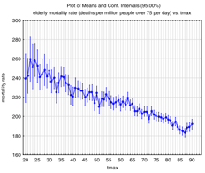 bstract of that paper, “Increases in average daily temperatures appear to significantly reduce average daily mortality rates, as expected from previous research.” Here is their plot of daily mortality rate versus Max temperature. It is clear that as the maximum temperature in a city goes up, mortality goes down. So if the net effect of increasing CO2 is increasing temperature, there should be a reduction in deaths.
I have a very large California data set. The data covers eight air basins and the years 2000 to 2012. There are over 37,000 exposure days and over two million deaths. The data for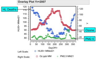 Los Angeles for the year 2007 is typical.
The number of Heart or Lung deaths for people 65 and older are given on the left, y-axis. The moving 21-day median number of deaths are given with blue diamonds as time marches to the right. Deaths are high during the winter, when temperatures are lower; the number of deaths are lower during the summer, when the temperatures are higher. These plots are typical. It is known that higher temperatures are associated with lower deaths.
A purported co-benefit of lower CO2 is that there will be lower levels of PM2.5. (PM2.5 is not chemically defined, but is partially made up of combustion products.) It is widely believed that lower levels of PM2.5 will lead to fewer deaths. Here is what Cox et al. (2013) have to say, “Unexpectedly, reductions in PM2.5 do not appear to cause any reductions in mortality rates.” And here is their supporting figure below.
Chay et al. (2003) looked at  a reduction in air pollution due to the Clean Air Act. Counties out of compliance were given stricter air pollution reduction goals. This action by the EPA created a so called natural experiment, Craig et al. (2012). The EPA selected counties did reduce air pollution levels, but there was no reduction in deaths after adjustments for covariates. Chay et al. (2003) say, “We find that regulatory status is associated with large reductions in TSPs pollution but has little association with reductions in either adult or elderly mortality.” So Cox et al. (2013) confirm the finding of Chay et al. (2003) that a reduction in PM2.5 does not lead to a reduction in deaths. Young and Xia (2013) found no assocation of PM2.5 with longevity in western US. Enstrom (2005) and many others have found no association of chronic deaths with PM2.5 in California.
Many claim an assocation of air pollution with deaths, acute and chronic. How can the two sets of claims be understood? Well, it depends. Greven et al. (2011) say in their abstract, “… we derive a Poisson regression model and estimate two regression coefficients: the “global” coefficient that measures the association between national trends in pollution and mortality; and the “local” coefficient, derived from space by time variation, that measures the association between location-specific trends in pollution and mortality adjusted by the national trends. …Results based on the global coefficient indicate a large increase in the national life expectancy for reductions in the yearly national average of PM2.5. However, this coefficient based on national trends in PM2.5 and mortality is likely to be confounded by other variables trending on the national level. Confounding of the local coefficient by unmeasured factors is less likely, although it cannot be ruled out. Based on the local coefficient alone, we are not able to demonstrate any change in life expectancy for a reduction in PM2.5.” (Italics mine) In plain words, associations measured from location to location, which are likely to be affected by differences in covariates, show an association. Examination of trends within locations, which are less likely to be affected by covariates, show no association. In short, the claims made depend on how well covariates are taken into account. When they are taken into account, Chay et al. (2003), Greven et al. (2011), Cox et al. (2013), Young (2014), there is no association of air pollution with deaths. Chay controls for multiple economic factors. Greven controls for location. Cox controls for temperature. Young controls for time and geography.
Note well: The analysis of Young (2014) uses a moving median within a location (air basin). This analysis is much less likely to be affected by covariates. This analysis finds no assocation of air pollution (PM2.5 or ozone) with deaths. Several figures are instructive. The figures are for LA, but are typical for the other California air basins. First ozone:
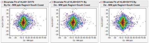
The figures were constructed as follows. From the daily death total was subtracted a 21-day moving median. This calculation corrects for the time trend in the data. From the daily air pollution level the 21-day moving median for the air pollution was subtracted. The daily death “deviation” was plotted against the pollution “deviation”. If air pollution was causing deaths, then the density in these three figures should go from lower left to upper right. To examine if previous air pollution, e.g. yesterday or the day before, was associated with current deaths, lags of 0, 1, and 2 days were used, hence the three figures. Plots like these were computed for all eight air basins; the figures for LA are typical. Next we give the same sort of figures, but for PM2.5. Again, LA.
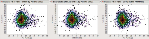
Again, the density is concentrated at zero PM2.5 and zero deaths, and, the important point, there is no tilt of the density from lower left to upper right. And again the plots for LA are typical of the other seven air basins.
Can we say more? Many authors have noted “geographic heterogeneity”, the measured effect of air pollution is not the same in different locations. There is overwhelming evidence for the existence of geographic heterogeneity. See for example, Krewski et al. (2000), Smith et al. (2009), Greven et al. (2011) and Young and Xia (2013). Multiple authors have not found any association of air pollution with acute deaths in California, Krewski et al. (2000), Smith et al. (2009), Young and Xia (2013) and Jarrett et al. (2013). Enstrom (2005) found no association with chronic deaths in California. A careful consideration of of this “geographic heterogeneity” is a key to understanding why it is unlikely that air pollution is causing deaths. Given that geographic heterogeneity exists, how should it be interpreted? First, statistical practice says that if interaction exists, then average effects often are misleading. Any recommendations should be for specific situations. In the words of the finance professor, it depends. In this case it makes no sense to regulate air pollution in California more severely than current regulations.
We can consider the question of interactions of air pollution with geography more deeply. Greven et al. (2011) state in their abstract, “Based on the local coefficient alone, we are not able to demonstrate any change in life expectancy for a reduction in PM2.5.” and they go on to say differences in locations (geographic heterogeneity) is most likely due to differences in covariates, e.g. age distributions, income, smoking. Indeed when Chay et al. (2003) corrected their analysis for an extensive list of covariates, they found no effect of the EPA intervention to reduce air pollution.
There is empirical evidence and a logical case that air pollution is (most likely) not causally related to acute deaths. Heart attacks and stroke were recently removed as a possible etiology, Milojevic et al. (2014).
Economics on the back of an envelope
The EPA claims saving 6,600 deaths per year due to CPP. They value each death at nine million dollars giving a co-benefit of $59.4B. But analysis that takes covariates into consideration finds no excess deaths due to ozone or PM2.5. The $59.4B co-benefit is the result of flawed analysis. And what is the cost of the regulation? The EPA says CPP is the most costly regulation it has considered and puts the cost at up to $90B/yr. The National Manufacturers Association puts the cost at $270B/yr, $900/person/year in 2020.
Consider Figure 4b of Young and Xia (2013). The data used in this figure is that used in Pope, Ezzati, and Dockery (2009) and was kindly provided by Arden Pope III. Change in income and air pollution from ~1980 to ~2000 was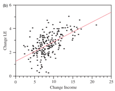 used. Income in thousands of dollars increase over that time period, but differed in magnitude from city to city, the x-axis. Life expectancy increased as well, y-axis. The general trend is very clear, increased income is associated with increased life expectancy. The income-life expectancy relationship is well-known. See the dramatic video by Hans Rosling (2010). To the extent that regulations are expensive, they should move people down and left in this figure with life expectancy less than it would have been. For example, $900 less income is expected to reduce life expectancy by two months.
So, do you want the EPA CPP regulations to extend your life not at all, costing you $900/yr or do you want to have use of your own money and save two months of your life? It depends. EPA decides or you decide.
Summary
- Increased CO2 is good for plants as plants grow better with increased CO2.
- Increases in temperature, however caused, are good for humans as they are less likely to die.
- The science literature, when covariates are controlled, is on the side that increased ozone and PM2.5 are not associated with increased deaths.
- On balance, the costs of reducing CO2, PM2.5 and ozone are expected to lead to reduced life expectancy.
Reblogged this on Power To The People and commented:
The Democrats don’t care about poor and black people. Their Green Dictatorship puts people in the poor house while they jet off to the next climate conference.
The Poisson Distribution describes rare phenomena.
The Poisson Distribution was used to describe horse-kicks in the Prussian Army and is useless for regression, which relies on the normal distribution.
True there is a transformation used to normalize the Poisson Distribution, but can you imagine the meaning of a correlation between horse-kicks in the Prussian Army with horse-kicks in the Polish Army?
That the EPA wishes to regulate substances related to rate phenomena would be equivalent to regulating the use of lightning rods. Sounds good in principle. But there is little or no evidence to support the intrusion of a government agency into this sphere of human activity.
We have reached and passed the point predicted by Alexis de Toqueville when he visited America. Government institutions are so strong that we have morphed from a people’s democracy to dictatorship of the majority called Bolshevism in Russian.
Totalitarian democracy has arrived and it wears the garb of the EPA. .